Has MMC changed? Completely different results on identical datasets

Good morning,

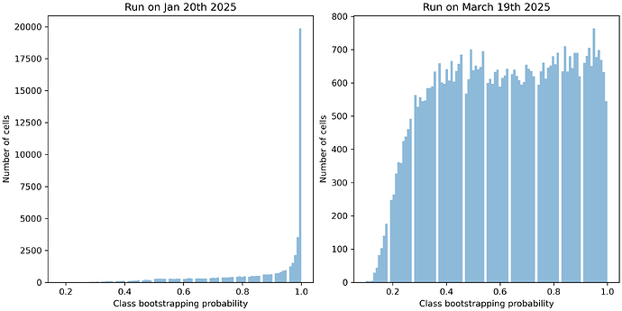
I was obtaining odd results with new datasets from mouse brain until I decided to resubmit an h5ad file that I had submitted 2 months ago. I am showing here the distribution of bootstrapping probability at the class level for the same h5ad file, the left one was run in January and the right one just today.

What has changed? The January results were very good.

EDIT: If this is of help here are the run IDs:
- Jan: 1737383574610
- March: 1742390354515

Any help will be much appreciated.

Best,
Matheu

Hi @MathieuBourdenx

The difference you are observing is due to a change we made in the default configuration parameters with which we run the MapMyCells algorithm (see this page and this webinar at around the 14 minute mark for a description of the MapMyCells algorithm).

At each level in the taxonomy, the bootstrapping_probability is determined as follows: we map each cell bootstrap_iteration times (bootstrap_iteration is a configurable integer >= 1), with each iteration using a random subset of bootstrap_factor of the whole set of marker genes (bootstrap_factor is a configurable parameter between that is > 0 and <= 1). We then choose the cell type that is selected by the plurality of the independent mapping iterations. The bootstrapping_probability is the fraction of iterations that chose the selected cell type. Ideally, low quality cells will have a low bootstrapping_probability, since the random subsampling of marker genes will result in a diversity of cell type assignments across iterations. High quality cells will have a high bootstrapping_probability, because data is so unambiguous that the change in marker gene subset will have little effect on the result of mapping.

Historically, we have run the algorithm with

bootstrap_iteration = 100
bootstrap_factor = 0.9

We have found that randomly subsetting 90% of the marker genes at each iteration did not yield a helpful value of bootstrapping_probability. 90% was so high that even low quality cells had a fairly consistent mapping and every cell had bootstrapping_probability > 0.9, regardless of quality.

Given that, we have adjusted the algorithm to use

bootstrap_iteraiton = 100
bootstrap_factor = 0.5

Now, each independent iteration of mapping has a more diverse set of marker genes, causing low quality cells to actually have a low bootstrapping_probability, an indication that the mapping may be suspect (depending on your tolerance for certainty of mapping).

For reference, you should be able to see these changes in configuration if you load the JSON output file and look at the metadata stored under the config key.

To offer a more concrete justification for this change:

The bootstrapping_probability at each level in the taxonomy can be thought of as a conditional probability (“the probability that the assignment that this level is correct, assuming that the assignments at the higher levels of the taxonomy are correct”). To get an unconditional probability, you can just take a running product of the probabilities starting at the highest level of the taxonomy (this is reported as the “aggregate_probability” in the JSON result file). With the change from bootstrap_factor=0.9 to bootstrap_factor=0.5, we found that the aggregate probability became a much better predictor of a mapping’s accuracy. When we performed a test-train hold out assessment using the Yao et al. transcriptomics data, we found that, for instance, if we took all the cells with aggregate_probability=0.6, roughly 60% of them were correct and 40% of them were incorrect (likewise, 20% of assignments with aggregate_probability=0.8 were incorrect). With bootstrap_factor=0.9, again, nearly every cell at every level had bootstrapping_probability > 0.9, regardless of whether or not the mapping was correct, so aggregate_probability really didn’t provide an easily interpretable metric for the quality of the mapping.

In our test-train evaluation, the change from bootstrap_factor=0.9 to bootstrap_factor=0.5 had almost no effect on the fraction of cells assigned to the correct cell type so, according to our tests, the only effect was that aggregate_probability became a better metric of quality.

So, in summary: while the bootstrapping_probability for your January run looked very good, that was deceptive. bootstrap_factor=0.9 is so large that even cells with a poor quality mapping received bootstrapping_probability ~ 1.0. I suspect that the new results actually reflect the quality of mapping for your cells.

Please let me know if you have any other questions or if anything is unclear.
Hi @danielsf,

Thanks a lot for your quick and detailed response. This makes a lot of sense!

One important aspect that I didn’t mention is that the data I am using are spatial transcriptomics data using the 500gene MERFISH panel from Yao et al. Have you validated to what extent this change in bootstrap_factor will affect cell-typing in spatial transcriptomic data? I can imagine that given the sparsity of the panel (and this would be an even higher problem with smaller gene panels where each cell-types only gets a handful of marker genes), bootstrap_factor will have an even higher impact on the bootstrapping probability.

What would you recommend? I can probably run MapMyCells locally using various bootstrap_factor.

Thanks a lot for your help!!

That is the $64,000 dollar question. In evaluating this change, we did test/train hold out with the Yao et al. 2023 single cell transcriptomic data (the only data for which we have anything approximating ground truth cell type assignments, since this is the data from which the Whole Mouse Brain taxonomy was derived). We modeled the effect of limited gene panels by taking the test data and randomly subsetting it to include different numbers of marker genes. We found that the effects of changing bootstrap_factor to 0.5 were roughly the same no matter how many marker genes were in the panel (so: quality of mapping was unaffected; quality of confidence estimate was improved). However, we found that panels with 500 genes in them were just terrible.

But: these were panels of 500 random genes. There’s a big difference between 500 random genes and the 500 genes chosen for a spatial transcriptomics panel because they mean something. If we used the 550 genes from the Yao et al. 2023 spatial transcriptomics data, the mapping was almost as good as if we included the full 32000 single cell gene panel.

We did not go as far as to simulate the effect of 500 well-chosen or commonly chosen spatial transcriptomics genes that weren’t the specific Yao et al. panel (which I believe was chosen to specifically include good markers for the Whole Mouse Brain taxonomy).

If you feel comfortable running the cell_type_mapper code locally in python (which it sounds like you do) this Jupyter notebook shows you how to download data from Yao et al. 2023, create a test set and a training set, map the test set, and evaluate the results. You could

  • download all of the Yao et al. 2023 data (fair warning, this will be ~ 200 GB)
  • create a test set from that data
  • downsample that test set to only include your 500 genes
  • map the downsampled dataset (either locally or on-line, depending on the size of the files) and see how accurate the mapping was so that you can get a sense of the accuracy you will get with your gene panel (Note that this does nothing to simulate any difference in noise distributions between spatial and single cell transcriptomics data).

If that sounds like a route you would like to pursue, I’m happy to provide any support for steps that become difficult.

Hi @danielsf,

Thanks for your reply. I do have the whole Yao et al. dataset already so what you suggest is definitely doable. I’ll report back once done!

Hi @danielsf,

Here are some results for what you suggested. I have randomly sampled 50k cells from the 4M in the Yao et al. 2023 taxonomy and mapped those with different values of bootstrap_factor (0.5, 0.6, 0.7, 0.8, 0.9). I repeated this process 50 times.
Here are the aggregated results.


There is an effect of the bootstrap factor on the F1 score, especially as we go deeper in the taxonomy. However, those results seem quite better than what I observe in spatial data. One possibility is that the sparsity of spatial data is higher and therefore impacting the cell-typing performance more.

What do you think? Any other ideas on how to further explore this?

Thanks!!!

Hi @MathieuBourdenx

Before talking about spatial data, I just want to make this quick aside (apologies if this is pedantic). The change that you are seeing in the F1 curves are, in my opinion, a reflection of the fact that the aggregate_probability is becoming a better reflection of how trustworthy a given cell’s mapping is. In the extreme case of bootstrap_factor=0.9, nearly every cell type mapping at every level in the taxonomy had bootstrap_probability >= 0.9, meaning that saying “I will only trust mappings with aggregate_probability >= 0.5” ends up distrusting (i.e. treating as incorrectly labeled) very few cells, which is why the F1 curve remains flat so far along the horizontal axis for high values of bootstrap_factor. There just isn’t much difference between cutting at aggregate_probability >= 0.5 and cutting at aggregate_probability >= 0.75, for instance. For lower bootstrap_factor values, drawing a cut in aggregate_probability actually does end up distrusting cells, introducing false negatives, and causing F1 to fall off as a function of aggregate_probability. When I said before that “changing bootstrap_factor to 0.5 had no appreciable affect in accuracy,” I was referring to the fact that the F1 curves at aggregate_probability = 0.0 (corresponding to “I trust all the cells, regardless of aggregate_probability”) do not change as a function of bootstrap_factor.

A corollary plot I like to produce to test my hypothesis (that aggregate_probability is becoming a better reflection of a mapping’s accuracy) is a plot of the theoretical versus actual cumulative distribution of correct mappings.

For a given value of x, take all the cells with aggregate_probability >= x. Sum up the aggregate_probability values of the selected cells. This is the number of correct assignments you would expect if the cell’s aggregate_probability values mean what they say (i.e. if 20% of cells with aggregate_probability=0.8 are wrong). Then, sum up the number of selected cells that actually were assigned their true cell types. This is the actual number of correct assignments. My argument is that, if aggregate_probability is a good measure of the confidence we should have in a cell’s mapping, the actual and expected number of correct assignments should be very close.

Seeing how the two curves (expected and actual correct assignments) evolve as a function of x for different values of bootstrap_factor is a way to assess what value of bootstrap_factor gives the best performance with respect to characterizing confidence in a cell’s mapping.

Spatial transcriptomics:

You are correct that the sparsity of the data could be a contributing factor. (Full disclosure: I am an astronomer by training, so I don’t know how to think about the noise profiles in transcriptomics data). If there was a way for you to simulate the sparsity of spatial transcriptomics data in the Yao et al. single cell data, you could see how increasing the sparsity affects the quality of the mapping.

The problem could also be that your gene panel does not contain enough of the pre-defined marker genes for the Whole Mouse Brain taxonomy. Since you have already downloaded the full Yao et al. reference dataset, it might be worthwhile for you to try creating your own set of marker genes that is customized to your spatial transcriptomics gene panel.

Section 5 of this Jupyter notebook shows how to go about selecting a new panel of marker genes. Both the ReferenceMarkerRunner and QueryMarkerRunner take an optional configuration parameter query_path which can point to the .h5ad file that contains your unlabeled data. If you use this parameter, the code will only select marker genes from the gene panel in your unlabeled data (there is a step in marker gene selection where combinatorics are used to select “the smallest useful set of marker genes,” but that step assumes that all genes in the Yao et al. reference data are valid choices; specifying query_path makes sure that only genes from your gene panel are considered when putting together this “smallest” set of markers).

I know that’s a lot to think about. I’m happy to answer any other questions you have.

1 Like